MixedNB Equivalence with GaussianNB

This example demonstrates that skbn.mixed_nb.MixedNB produces identical results to sklearn.naive_bayes.GaussianNB when all features are continuous (Gaussian).

The plot shows the decision boundaries for both classifiers. As expected, the boundaries are identical, and the predicted probabilities for the dataset are all-close.

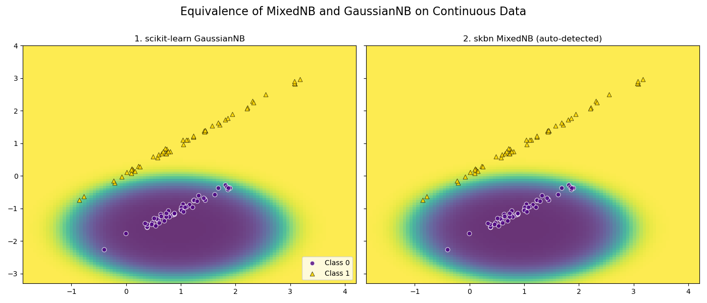
GaussianNB vs MixedNB Equivalence Check: Probabilities are identical.

# Author: The scikit-bayes Developers
# SPDX-License-Identifier: BSD-3-Clause

import matplotlib.pyplot as plt
from numpy.testing import assert_allclose
from sklearn.datasets import make_classification
from sklearn.inspection import DecisionBoundaryDisplay
from sklearn.naive_bayes import GaussianNB

from skbn.mixed_nb import MixedNB

# 1. Generate a 2D Gaussian dataset
X, y = make_classification(
    n_samples=100,
    n_features=2,
    n_informative=2,
    n_redundant=0,
    n_clusters_per_class=1,
    random_state=42,
)

# 2. Fit both classifiers
gnb = GaussianNB()
gnb.fit(X, y)
probs_gnb = gnb.predict_proba(X)

# MixedNB will auto-detect both features as 'gaussian'
mnb = MixedNB()
mnb.fit(X, y)
probs_mnb = mnb.predict_proba(X)

# 3. Assert equivalence
try:
    assert_allclose(probs_gnb, probs_mnb, rtol=1e-7, atol=1e-7)
    equivalence_message = "Probabilities are identical."
except AssertionError as e:
    equivalence_message = f"Probabilities are NOT identical:\n{e}"

print(f"GaussianNB vs MixedNB Equivalence Check: {equivalence_message}")

# 4. Plot decision boundaries
fig, axes = plt.subplots(1, 2, figsize=(14, 6), sharey=True)

models = [gnb, mnb]
titles = ["1. scikit-learn GaussianNB", "2. skbn MixedNB (auto-detected)"]

for ax, model, title in zip(axes, models, titles):
    # Plot Decision Boundary - VIRIDIS
    DecisionBoundaryDisplay.from_estimator(
        model,
        X,
        ax=ax,
        response_method="predict_proba",
        plot_method="pcolormesh",
        shading="auto",
        alpha=0.8,
        cmap="viridis",
    )

    # Overlay real data points with consistent style
    # Class 0 -> Indigo
    ax.scatter(
        X[y == 0, 0],
        X[y == 0, 1],
        c="indigo",
        marker="o",
        s=40,
        alpha=0.8,
        edgecolors="w",
        linewidth=0.8,
        label="Class 0",
    )

    # Class 1 -> Gold
    ax.scatter(
        X[y == 1, 0],
        X[y == 1, 1],
        c="gold",
        marker="^",
        s=40,
        alpha=0.9,
        edgecolors="k",
        linewidth=0.5,
        label="Class 1",
    )

    ax.set_title(title, fontsize=12)

# Add Legend to the first plot
axes[0].legend(loc="lower right")

fig.suptitle("Equivalence of MixedNB and GaussianNB on Continuous Data", fontsize=16)
plt.tight_layout()
plt.subplots_adjust(top=0.85)
plt.show()