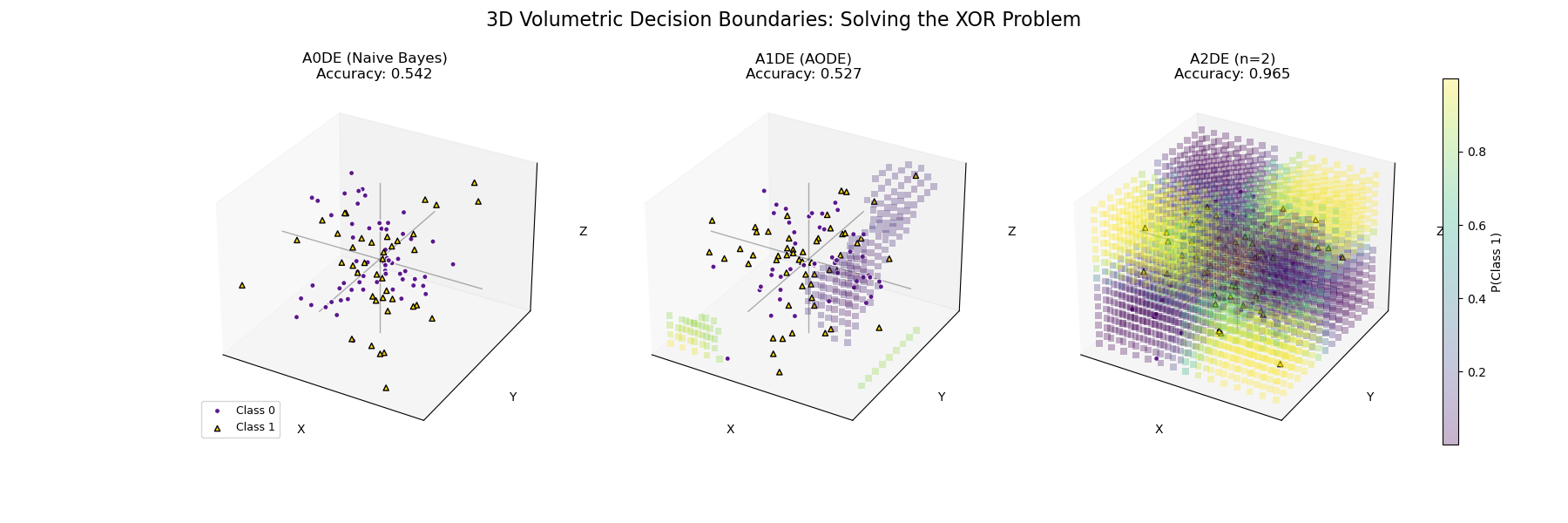
3D Voxel-Cloud Visualization: XOR Structure

To visualize the 3D decision boundaries clearly, we plot a dense cloud of points (voxels) colored by the predicted class probability.

This reveals the internal geometry of the classifier: - A0DE: Shows a uniform blob (fails to separate). Accuracy ~0.5. - A1DE: Also fails to find structure (linear/planar cuts insufficient for 3D parity). Accuracy ~0.5. - A2DE: Shows a distinct 3D Checkerboard pattern (perfect solution).

Training models...
Generating volumetric grid...

# Author: The scikit-bayes Developers
# SPDX-License-Identifier: BSD-3-Clause

import matplotlib.pyplot as plt
import numpy as np
from mpl_toolkits.mplot3d import Axes3D  # noqa: F401
from sklearn.metrics import accuracy_score

from skbn.ande import AnDE
from skbn.mixed_nb import MixedNB

# --- 1. Generate 3D XOR Dataset ---
np.random.seed(42)
n_samples = 2000
X = np.random.randn(n_samples, 3)
# 3D Parity Logic: Class 1 if product of signs is positive
y = (np.sign(X[:, 0]) * np.sign(X[:, 1]) * np.sign(X[:, 2]) > 0).astype(int)

# --- 2. Fit Models ---
print("Training models...")
models = [MixedNB(), AnDE(n_dependence=1, n_bins=4), AnDE(n_dependence=2, n_bins=4)]
names = ["A0DE (Naive Bayes)", "A1DE (AODE)", "A2DE (n=2)"]

fitted_models = []
scores = []
for model in models:
    model.fit(X, y)
    acc = accuracy_score(y, model.predict(X))
    fitted_models.append(model)
    scores.append(acc)

# --- 3. Generate Prediction Grid ---
print("Generating volumetric grid...")
# Create a simpler grid for visualization (less dense than before for clarity)
n_grid = 15
grid_range = np.linspace(-2.2, 2.2, n_grid)
xx, yy, zz = np.meshgrid(grid_range, grid_range, grid_range)
X_grid = np.column_stack([xx.ravel(), yy.ravel(), zz.ravel()])

# --- 4. Plotting ---
fig = plt.figure(figsize=(18, 6))

for i, (model, name, score) in enumerate(zip(fitted_models, names, scores)):
    ax = fig.add_subplot(1, 3, i + 1, projection="3d")

    # Predict probabilities
    probs = model.predict_proba(X_grid)[:, 1]

    # Visualization Trick:
    # Plot points where the model is confident.
    # High prob (Yellow) and Low prob (Purple).
    mask = np.abs(probs - 0.5) > 0.1

    xs = X_grid[mask, 0]
    ys = X_grid[mask, 1]
    zs = X_grid[mask, 2]
    c_vals = probs[mask]

    # 1. Plot Voxel Cloud (Model Belief)
    # cmap='viridis' matches our theme: 0 (Purple) -> 1 (Yellow)
    p = ax.scatter(
        xs,
        ys,
        zs,
        c=c_vals,
        cmap="viridis",
        s=30,
        alpha=0.3,
        edgecolors="none",
        marker="s",
    )

    # 2. Overlay Real Data Points (Ground Truth)
    # Subsample to avoid cluttering the 3D view
    mask_sub = np.random.choice(n_samples, 100, replace=False)
    X_sub = X[mask_sub]
    y_sub = y[mask_sub]

    # Class 0 -> Indigo Circle
    ax.scatter(
        X_sub[y_sub == 0, 0],
        X_sub[y_sub == 0, 1],
        X_sub[y_sub == 0, 2],
        c="indigo",
        marker="o",
        s=20,
        alpha=0.9,
        edgecolors="w",
        label="Class 0",
    )

    # Class 1 -> Gold Triangle
    ax.scatter(
        X_sub[y_sub == 1, 0],
        X_sub[y_sub == 1, 1],
        X_sub[y_sub == 1, 2],
        c="gold",
        marker="^",
        s=20,
        alpha=1.0,
        edgecolors="k",
        label="Class 1",
    )

    # Add axes lines crossing at zero for reference
    ax.plot([-2.5, 2.5], [0, 0], [0, 0], "k-", lw=1, alpha=0.3)
    ax.plot([0, 0], [-2.5, 2.5], [0, 0], "k-", lw=1, alpha=0.3)
    ax.plot([0, 0], [0, 0], [-2.5, 2.5], "k-", lw=1, alpha=0.3)

    ax.set_title(f"{name}\nAccuracy: {score:.3f}", fontsize=12)
    ax.set_xlabel("X")
    ax.set_ylabel("Y")
    ax.set_zlabel("Z")

    # Cleaner look
    ax.set_xticks([])
    ax.set_yticks([])
    ax.set_zticks([])
    ax.set_xlim(-2.5, 2.5)
    ax.set_ylim(-2.5, 2.5)
    ax.set_zlim(-2.5, 2.5)

# Add colorbar
cbar_ax = fig.add_axes([0.92, 0.15, 0.01, 0.7])
fig.colorbar(p, cax=cbar_ax, label="P(Class 1)")

# Add legend to the first plot only (to save space)
axes_3d = fig.get_axes()[0]
axes_3d.legend(loc="lower left", fontsize=9)

plt.suptitle("3D Volumetric Decision Boundaries: Solving the XOR Problem", fontsize=16)
plt.show()