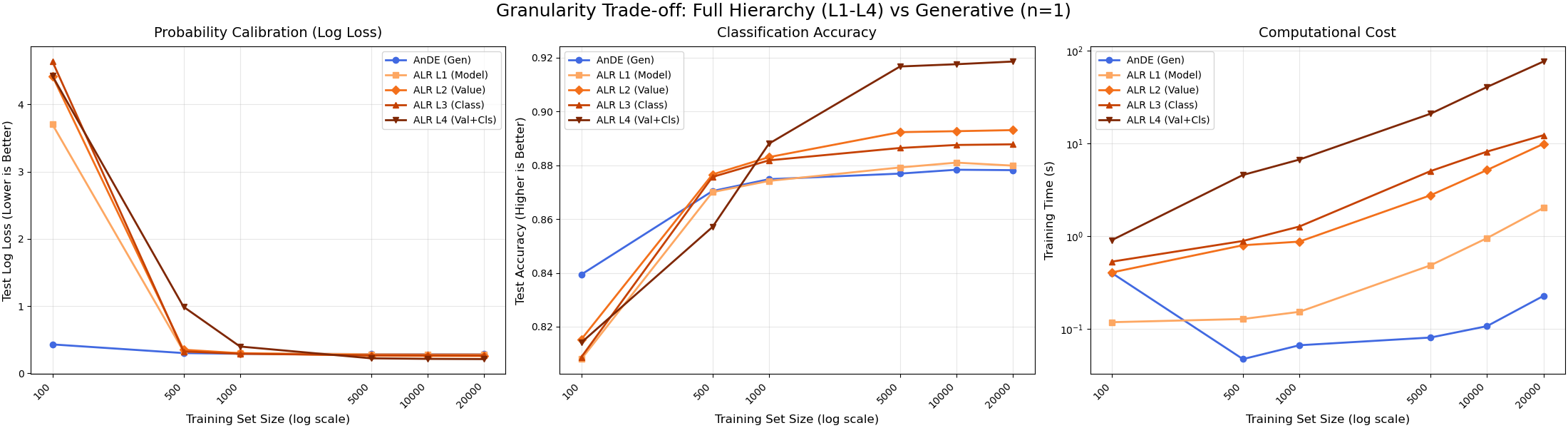
Data Efficiency & Complexity: Generative vs. Hybrid Levels (L1-L4)

This experiment compares the full hierarchy of parameter granularity in ALR.

Models Compared: 1. AnDE (Generative): Baseline. No weights. 2. ALR Level 1 (Model): 1 weight per SPODE. (Low Variance). 3. ALR Level 2 (Value): 1 weight per SPODE per Parent Value. (High Variance). 4. ALR Level 3 (Class): 1 weight per SPODE per Class. (Balanced). 5. ALR Level 4 (Val+Cls): 1 weight per SPODE per Parent Value per Class. (Max Variance).

Observations: - Small N (~200): AnDE (Generative) leads due to better calibration. Hybrids may overfit. - Medium N (~500): ALR (Hybrid) catches up. - Large N (>5000): Higher granularity wins. Order: L1 < L2 < L3 < L4. - Time: L4 is significantly slower due to larger optimization space.

Running benchmark with all 4 granularity levels...
Seed 1, N=100 done.
Seed 1, N=500 done.
Seed 1, N=1000 done.
Seed 1, N=5000 done.
Seed 1, N=10000 done.
Seed 1, N=20000 done.
Seed 2, N=100 done.
Seed 2, N=500 done.
Seed 2, N=1000 done.
Seed 2, N=5000 done.
Seed 2, N=10000 done.
Seed 2, N=20000 done.
Seed 3, N=100 done.
Seed 3, N=500 done.
Seed 3, N=1000 done.
Seed 3, N=5000 done.
Seed 3, N=10000 done.
Seed 3, N=20000 done.
Seed 42, N=100 done.
Seed 42, N=500 done.
Seed 42, N=1000 done.
Seed 42, N=5000 done.
Seed 42, N=10000 done.
Seed 42, N=20000 done.
Seed 123, N=100 done.
Seed 123, N=500 done.
Seed 123, N=1000 done.
Seed 123, N=5000 done.
Seed 123, N=10000 done.
Seed 123, N=20000 done.

# Author: The scikit-bayes Developers
# SPDX-License-Identifier: BSD-3-Clause

import time

import matplotlib.pyplot as plt
import numpy as np
from matplotlib.ticker import ScalarFormatter
from sklearn.datasets import make_classification
from sklearn.metrics import accuracy_score, log_loss
from sklearn.model_selection import train_test_split

from skbn.ande import ALR, AnDE

# Setup
seeds = [1, 2, 3, 42, 123]
# Full range of sizes to see the crossover
sizes = [100, 500, 1000, 5000, 10000, 20000]

models_config = [
    ("AnDE (Gen)", lambda: AnDE(n_dependence=1, n_jobs=-1)),
    (
        "ALR L1 (Model)",
        lambda: ALR(n_dependence=1, weight_level=1, l2_reg=1e-3, n_jobs=-1),
    ),
    (
        "ALR L2 (Value)",
        lambda: ALR(n_dependence=1, weight_level=2, l2_reg=1e-3, n_jobs=-1),
    ),
    (
        "ALR L3 (Class)",
        lambda: ALR(n_dependence=1, weight_level=3, l2_reg=1e-3, n_jobs=-1),
    ),
    (
        "ALR L4 (Val+Cls)",
        lambda: ALR(n_dependence=1, weight_level=4, l2_reg=1e-3, n_jobs=-1),
    ),
]

# Results storage: [seed, size, model]
n_models = len(models_config)
res_ll = np.zeros((len(seeds), len(sizes), n_models))
res_acc = np.zeros((len(seeds), len(sizes), n_models))
res_time = np.zeros((len(seeds), len(sizes), n_models))

print("Running benchmark with all 4 granularity levels...")

for i, seed in enumerate(seeds):
    # Using a slightly larger dataset to ensure we have enough for the biggest train split
    X, y = make_classification(
        n_samples=30000, n_features=10, n_informative=8, random_state=seed
    )

    for j, n_train in enumerate(sizes):
        X_train, X_test, y_train, y_test = train_test_split(
            X, y, train_size=n_train, test_size=5000, random_state=seed
        )

        for k, (name, factory) in enumerate(models_config):
            clf = factory()

            start = time.time()
            clf.fit(X_train, y_train)
            res_time[i, j, k] = time.time() - start

            # Use predict_proba for both metrics to save one inference pass if wanted,
            # but predict() is safer for accuracy consistency.
            y_prob = clf.predict_proba(X_test)
            y_pred = clf.predict(X_test)

            res_ll[i, j, k] = log_loss(y_test, y_prob)
            res_acc[i, j, k] = accuracy_score(y_test, y_pred)

        print(f"Seed {seed}, N={n_train} done.")

# Average
mean_ll = res_ll.mean(axis=0)
mean_acc = res_acc.mean(axis=0)
mean_time = res_time.mean(axis=0)

# --- Visualization ---
fig, axes = plt.subplots(1, 3, figsize=(22, 6), layout="constrained")

# Define Colors:
# AnDE gets a unique cool color.
# ALR levels get a warm sequential gradient (Light Orange -> Dark Red/Brown)
cmap = plt.cm.Oranges
# Generate 4 colors from the colormap, starting from 0.4 to avoid too light colors
alr_colors = [cmap(x) for x in np.linspace(0.4, 1.0, 4)]
colors = ["royalblue"] + alr_colors

# Markers: Distinct shapes
markers = ["o", "s", "D", "^", "v"]

for k, (name, _) in enumerate(models_config):
    # Plot 1: Log Loss
    axes[0].plot(
        sizes,
        mean_ll[:, k],
        marker=markers[k],
        label=name,
        color=colors[k],
        lw=2,
        markersize=6,
    )
    # Plot 2: Accuracy
    axes[1].plot(
        sizes,
        mean_acc[:, k],
        marker=markers[k],
        label=name,
        color=colors[k],
        lw=2,
        markersize=6,
    )
    # Plot 3: Training Time
    axes[2].plot(
        sizes,
        mean_time[:, k],
        marker=markers[k],
        label=name,
        color=colors[k],
        lw=2,
        markersize=6,
    )

# --- Formatting ---

# Panel 1: Log Loss
axes[0].set_ylabel("Test Log Loss (Lower is Better)", fontsize=12)
axes[0].set_title("Probability Calibration (Log Loss)", fontsize=14, pad=10)

# Panel 2: Accuracy
axes[1].set_ylabel("Test Accuracy (Higher is Better)", fontsize=12)
axes[1].set_title("Classification Accuracy", fontsize=14, pad=10)

# Panel 3: Time
axes[2].set_ylabel("Training Time (s)", fontsize=12)
axes[2].set_title("Computational Cost", fontsize=14, pad=10)
axes[2].set_yscale("log")

# Common formatting for all subplots
for ax in axes:
    ax.set_xlabel("Training Set Size (log scale)", fontsize=12)
    ax.set_xscale("log")
    ax.grid(True, which="major", ls="-", alpha=0.3)
    ax.legend(fontsize=10, loc="best")

    # --- FIX: Readable X-Axis Labels ---
    # 1. Force matplotlib to use exactly our dataset sizes as ticks
    ax.set_xticks(sizes)

    # 2. Format as plain integers (e.g., 100, 500) instead of scientific (1e2)
    ax.get_xaxis().set_major_formatter(ScalarFormatter())

    # 3. Rotate labels to prevent horizontal overlapping
    ax.set_xticklabels(sizes, rotation=45, ha="right")

    # 4. Remove minor ticks to clean up the log-scale look
    ax.minorticks_off()

# Global Title
fig.suptitle(
    "Granularity Trade-off: Full Hierarchy (L1-L4) vs Generative (n=1)", fontsize=18
)

plt.show()