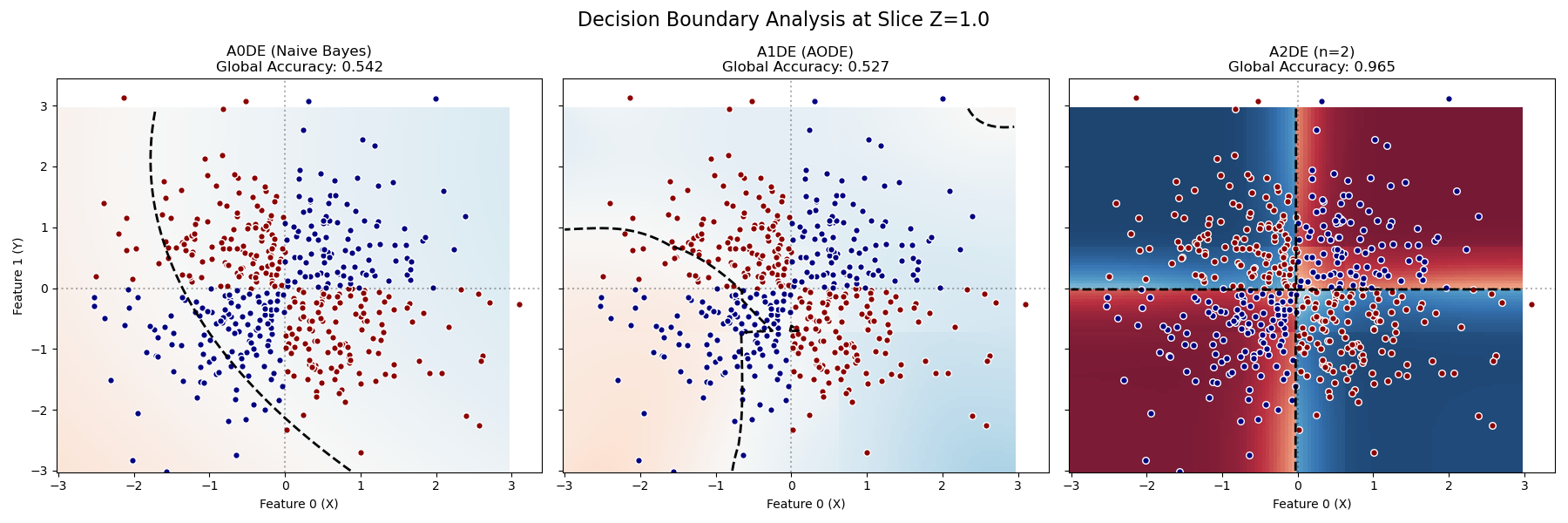
Analytic View: 2D Slice of the 3D XOR Problem

While 3D visualizations show the global structure, taking a 2D slice (fixing one feature) allows for a precise analysis of the decision boundary.

Here we fix $z = 1.0$. In the 3D XOR problem $(x oplus y oplus z)$, if $z$ is positive (True), the logic simplifies to a standard 2D XOR between $x$ and $y$: $(x oplus y oplus 1) ightarrow eg(x oplus y)$ (XNOR behavior).

What to look for:

1. A0DE (NB): Blurry background, no structure. Accuracy ~0.5 (Random).

2. A1DE (AODE): Might show vertical or horizontal stripes, but fails to capture the checkerboard. Accuracy ~0.5 (Random).

3. A2DE (n=2): Shows a distinct “Checkerboard” pattern with sharp boundaries. Accuracy ~0.965 (Solved).

Training models...

# Author: The scikit-bayes Developers
# SPDX-License-Identifier: BSD-3-Clause

import matplotlib.pyplot as plt
import numpy as np
from sklearn.metrics import accuracy_score

from skbn.ande import AnDE
from skbn.mixed_nb import MixedNB

# --- 1. Generate 3D XOR Dataset ---
np.random.seed(42)
n_samples = 2000
X = np.random.randn(n_samples, 3)
# Logic: Product of signs > 0 -> Class 1
y = (np.sign(X[:, 0]) * np.sign(X[:, 1]) * np.sign(X[:, 2]) > 0).astype(int)

# --- 2. Fit Models ---
print("Training models...")
models = [MixedNB(), AnDE(n_dependence=1, n_bins=4), AnDE(n_dependence=2, n_bins=4)]
names = ["A0DE (Naive Bayes)", "A1DE (AODE)", "A2DE (n=2)"]

for model in models:
    model.fit(X, y)

# --- 3. Visualization Setup ---
fig, axes = plt.subplots(1, 3, figsize=(18, 6), sharey=True)

# Grid for Z=1 slice
h = 0.05
limit = 3
xx, yy = np.meshgrid(np.arange(-limit, limit, h), np.arange(-limit, limit, h))
grid_flat = np.c_[xx.ravel(), yy.ravel()]
# Construct query points (x, y, 1.0)
X_test_slice = np.hstack([grid_flat, np.ones((len(grid_flat), 1))])

for ax, model, name in zip(axes, models, names):
    # Global Accuracy
    acc = accuracy_score(y, model.predict(X))

    # Probabilities on the slice
    probs = model.predict_proba(X_test_slice)[:, 1]
    Z_probs = probs.reshape(xx.shape)

    # A. Plot Probability Background (Diverging Colormap)
    # RdBu_r: Red (Class 0) <--> White (0.5) <--> Blue (Class 1)
    # This clearly shows confidence and the decision boundary
    cf = ax.pcolormesh(
        xx, yy, Z_probs, cmap="RdBu_r", vmin=0, vmax=1, shading="auto", alpha=0.9
    )

    # B. Add Contour Line for Decision Boundary
    ax.contour(
        xx, yy, Z_probs, levels=[0.5], colors="black", linewidths=2, linestyles="--"
    )

    # C. Overlay Data Points (Only those near the slice Z=1)
    # We take a slice z in [0.5, 1.5] to represent the volume being projected
    mask_slice = (X[:, 2] > 0.5) & (X[:, 2] < 1.5)

    # Plot Class 0 (Red dots) vs Class 1 (Blue dots) to match colormap
    ax.scatter(
        X[mask_slice & (y == 0), 0],
        X[mask_slice & (y == 0), 1],
        c="darkred",
        edgecolors="w",
        s=30,
        label="Class 0",
    )
    ax.scatter(
        X[mask_slice & (y == 1), 0],
        X[mask_slice & (y == 1), 1],
        c="navy",
        edgecolors="w",
        s=30,
        label="Class 1",
    )

    ax.set_title(f"{name}\nGlobal Accuracy: {acc:.3f}")
    ax.set_xlabel("Feature 0 (X)")

    # Quadrant reference lines
    ax.axvline(0, color="k", linestyle=":", alpha=0.3)
    ax.axhline(0, color="k", linestyle=":", alpha=0.3)

axes[0].set_ylabel("Feature 1 (Y)")
fig.suptitle("Decision Boundary Analysis at Slice Z=1.0", fontsize=16)
plt.tight_layout()
plt.subplots_adjust(top=0.85)
plt.show()