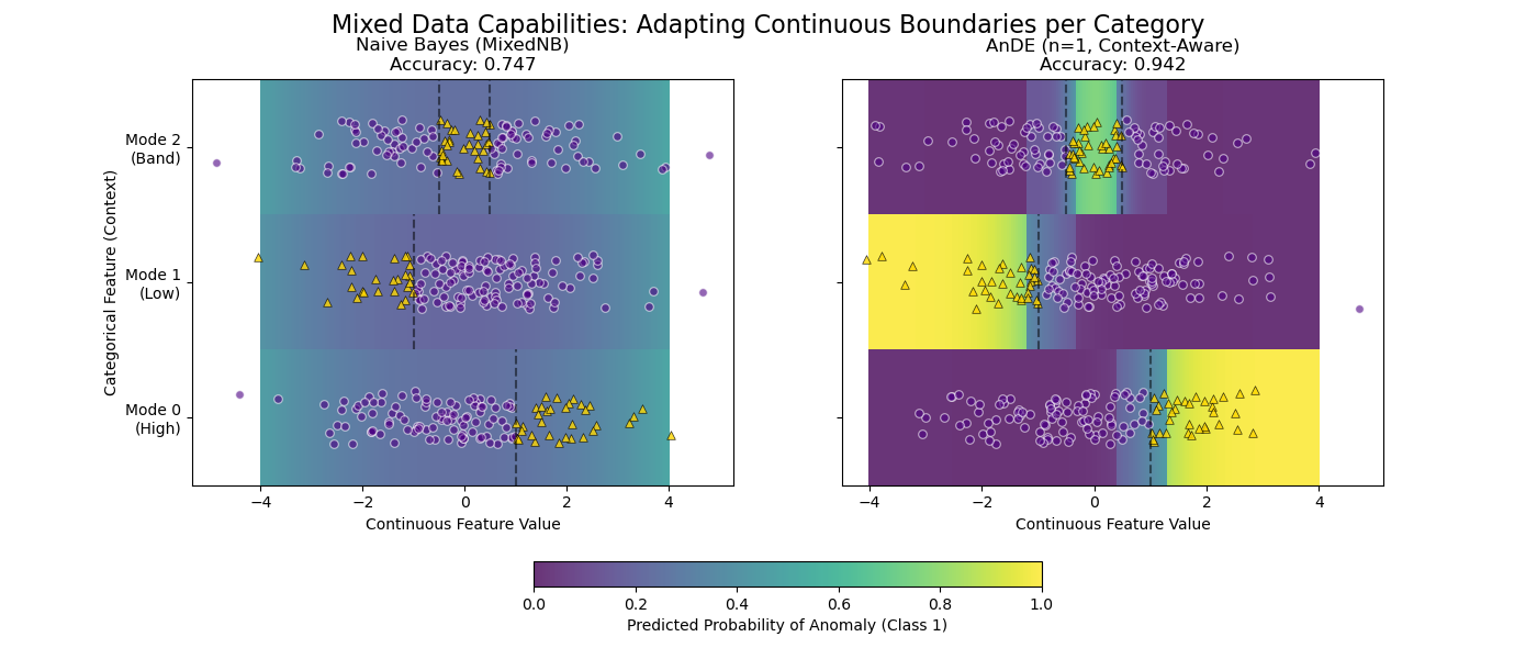
The Power of Mixed Data: Context-Dependent Logic

This example demonstrates why AnDE shines with mixed data types (Continuous + Categorical) compared to Naive Bayes.

We simulate a system with a Continuous Feature (X) and a Categorical “Mode” (C). The definition of “Anomaly” (Class 1) changes completely depending on the mode.

Result: - MixedNB (Naive): Fails. It smears probability across the range. - AnDE (n=1): Succeeds. It learns distinct boundaries per mode.

Training models...

# Author: The scikit-bayes Developers
# SPDX-License-Identifier: BSD-3-Clause

import warnings

import matplotlib.pyplot as plt
import numpy as np
from sklearn.metrics import accuracy_score

from skbn.ande import AnDE
from skbn.mixed_nb import MixedNB

# Suppress discretization warnings for this demo
warnings.filterwarnings("ignore", category=UserWarning)

# --- 1. Generate Mixed Dataset ---
np.random.seed(42)
n_samples = 3000

# Feature 0: Continuous (Standard Normal)
X_cont = np.random.randn(n_samples, 1) * 1.5
# Feature 1: Categorical (0, 1, 2)
X_cat = np.random.randint(0, 3, size=(n_samples, 1))

# Stack them
X = np.hstack([X_cont, X_cat])

# Logic:
y = np.zeros(n_samples, dtype=int)
# Mode 0: Positive High (> 1)
mask_0 = (X_cat.flatten() == 0) & (X_cont.flatten() > 1.0)
y[mask_0] = 1
# Mode 1: Positive Low (< -1)
mask_1 = (X_cat.flatten() == 1) & (X_cont.flatten() < -1.0)
y[mask_1] = 1
# Mode 2: Positive Middle (-0.5 < x < 0.5)
mask_2 = (X_cat.flatten() == 2) & (np.abs(X_cont.flatten()) < 0.5)
y[mask_2] = 1

# --- 2. Fit Models ---
print("Training models...")

mnb = MixedNB()
mnb.fit(X, y)

ande = AnDE(n_dependence=1)
ande.fit(X, y)

models = [mnb, ande]
titles = ["Naive Bayes (MixedNB)", "AnDE (n=1, Context-Aware)"]

# --- 3. Visualization ---
fig, axes = plt.subplots(1, 2, figsize=(14, 6), sharey=True)

# Grid for plotting
# We need CENTERS for prediction, but EDGES for pcolormesh plotting
n_points = 200
x_centers = np.linspace(-4, 4, n_points)

# Create edges for X (must be length n_points + 1)
step = x_centers[1] - x_centers[0]
x_edges = np.concatenate([x_centers - step / 2, [x_centers[-1] + step / 2]])

# Y edges are manual (categorical bands)
y_edges = np.array([-0.5, 0.5, 1.5, 2.5])

# Prediction loop
for ax, model, title in zip(axes, models, titles):
    acc = accuracy_score(y, model.predict(X))

    # Construct probability map
    prob_map = np.zeros((3, n_points))

    for cat_val in [0, 1, 2]:
        # Create a batch of data: [x_centers, constant_cat]
        batch_cat = np.full((n_points, 1), cat_val)
        batch_X = np.hstack([x_centers.reshape(-1, 1), batch_cat])

        # Predict
        probs = model.predict_proba(batch_X)[:, 1]
        prob_map[cat_val, :] = probs

    # Plot Heatmap - VIRIDIS
    # cmap='viridis': Purple (0.0) -> Yellow (1.0)
    pcm = ax.pcolormesh(
        x_edges,
        y_edges,
        prob_map,
        cmap="viridis",
        vmin=0,
        vmax=1,
        shading="flat",
        alpha=0.8,
    )

    # Overlay real data points
    mask_sub = np.random.choice(n_samples, 400, replace=False)
    X_sub = X[mask_sub]
    y_sub = y[mask_sub]

    # Jitter Y for visibility
    y_jitter = X_sub[:, 1] + np.random.uniform(-0.2, 0.2, size=len(X_sub))

    # Class 0 -> Indigo Circle (Low prob)
    ax.scatter(
        X_sub[y_sub == 0, 0],
        y_jitter[y_sub == 0],
        c="indigo",
        marker="o",
        s=30,
        alpha=0.6,
        edgecolors="w",
        linewidth=0.8,
        label="Class 0",
    )

    # Class 1 -> Gold Triangle (High prob)
    # Black edge for contrast against yellow background
    ax.scatter(
        X_sub[y_sub == 1, 0],
        y_jitter[y_sub == 1],
        c="gold",
        marker="^",
        s=30,
        alpha=0.8,
        edgecolors="k",
        linewidth=0.5,
        label="Class 1",
    )

    ax.set_title(f"{title}\nAccuracy: {acc:.3f}")
    ax.set_xlabel("Continuous Feature Value")
    ax.set_yticks([0, 1, 2])
    ax.set_yticklabels(["Mode 0\n(High)", "Mode 1\n(Low)", "Mode 2\n(Band)"])

    # Reference lines
    ax.vlines(1.0, -0.5, 0.5, colors="black", linestyles="--", alpha=0.5)
    ax.vlines(-1.0, 0.5, 1.5, colors="black", linestyles="--", alpha=0.5)
    ax.vlines([-0.5, 0.5], 1.5, 2.5, colors="black", linestyles="--", alpha=0.5)

axes[0].set_ylabel("Categorical Feature (Context)")
cbar = fig.colorbar(
    pcm, ax=axes.ravel().tolist(), orientation="horizontal", fraction=0.05, pad=0.15
)
cbar.set_label("Predicted Probability of Anomaly (Class 1)")

fig.suptitle(
    "Mixed Data Capabilities: Adapting Continuous Boundaries per Category", fontsize=16
)
plt.show()