MixedNB Equivalence with CategoricalNB

This example demonstrates that skbn.mixed_nb.MixedNB produces identical results to sklearn.naive_bayes.CategoricalNB when all features are discrete (categorical).

The plot shows the decision boundaries for both classifiers. As expected, the boundaries are identical, and the predicted probabilities for the dataset are all-close.

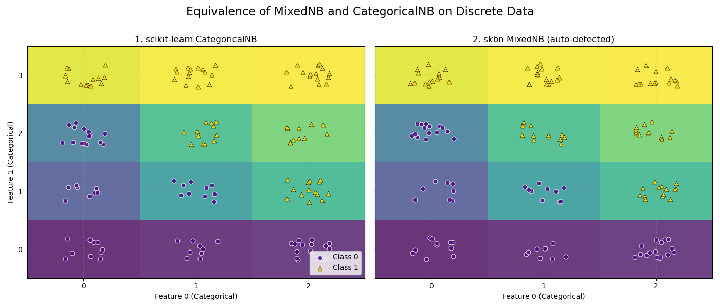
CategoricalNB vs MixedNB Equivalence Check: Probabilities are identical.

# Author: The scikit-bayes Developers
# SPDX-License-Identifier: BSD-3-Clause

import matplotlib.pyplot as plt
import numpy as np
from numpy.testing import assert_allclose
from sklearn.naive_bayes import CategoricalNB

from skbn.mixed_nb import MixedNB

# 1. Generate a 2D Categorical dataset (3 categories for f0, 4 for f1)
np.random.seed(42)
n_samples = 150
X = np.zeros((n_samples, 2), dtype=int)
X[:, 0] = np.random.randint(0, 3, size=n_samples)
X[:, 1] = np.random.randint(0, 4, size=n_samples)
# Logic: Interaction between categories
y = (X[:, 0] + X[:, 1] >= 3).astype(int)

# 2. Fit both classifiers
cnb = CategoricalNB(alpha=1.0)
cnb.fit(X, y)
probs_cnb = cnb.predict_proba(X)

# MixedNB will auto-detect both features as 'categorical'
mnb = MixedNB(alpha=1.0)
mnb.fit(X, y)
probs_mnb = mnb.predict_proba(X)

# 3. Assert equivalence
try:
    assert_allclose(probs_cnb, probs_mnb, rtol=1e-7, atol=1e-7)
    equivalence_message = "Probabilities are identical."
except AssertionError as e:
    equivalence_message = f"Probabilities are NOT identical:\n{e}"

print(f"CategoricalNB vs MixedNB Equivalence Check: {equivalence_message}")

# 4. Plot decision boundaries
fig, axes = plt.subplots(1, 2, figsize=(14, 6), sharey=True)

models = [cnb, mnb]
titles = ["1. scikit-learn CategoricalNB", "2. skbn MixedNB (auto-detected)"]

# Define grid for visualization (Centers for prediction, Edges for plotting)
# Feature 0: Categories 0, 1, 2
x_centers = np.arange(3)
x_edges = np.arange(4) - 0.5

# Feature 1: Categories 0, 1, 2, 3
y_centers = np.arange(4)
y_edges = np.arange(5) - 0.5

# Create prediction grid (Integer combinations)
xx, yy = np.meshgrid(x_centers, y_centers)
grid_pred = np.c_[xx.ravel(), yy.ravel()]

for ax, model, title in zip(axes, models, titles):
    # Predict probabilities on integer grid
    probs = model.predict_proba(grid_pred)[:, 1]
    Z = probs.reshape(xx.shape)

    # Plot Heatmap - VIRIDIS
    # Using pcolormesh with edges defines the "blocks" perfectly
    ax.pcolormesh(
        x_edges,
        y_edges,
        Z,
        cmap="viridis",
        vmin=0,
        vmax=1,
        shading="flat",
        alpha=0.8,
        edgecolors="none",
    )

    # Overlay real data points with consistent style
    # Jitter points slightly to show density
    x_jit = X[:, 0] + np.random.uniform(-0.2, 0.2, size=n_samples)
    y_jit = X[:, 1] + np.random.uniform(-0.2, 0.2, size=n_samples)

    # Class 0 -> Indigo Circle
    ax.scatter(
        x_jit[y == 0],
        y_jit[y == 0],
        c="indigo",
        marker="o",
        s=40,
        alpha=0.8,
        edgecolors="w",
        linewidth=0.8,
        label="Class 0",
    )

    # Class 1 -> Gold Triangle
    ax.scatter(
        x_jit[y == 1],
        y_jit[y == 1],
        c="gold",
        marker="^",
        s=40,
        alpha=0.9,
        edgecolors="k",
        linewidth=0.5,
        label="Class 1",
    )

    ax.set_title(title, fontsize=12)
    ax.set_xlabel("Feature 0 (Categorical)")
    ax.set_xticks(x_centers)
    ax.set_yticks(y_centers)
    ax.grid(True, alpha=0.2, linestyle="--")

axes[0].set_ylabel("Feature 1 (Categorical)")
axes[0].legend(loc="lower right")

fig.suptitle("Equivalence of MixedNB and CategoricalNB on Discrete Data", fontsize=16)
plt.tight_layout()
plt.subplots_adjust(top=0.85)
plt.show()