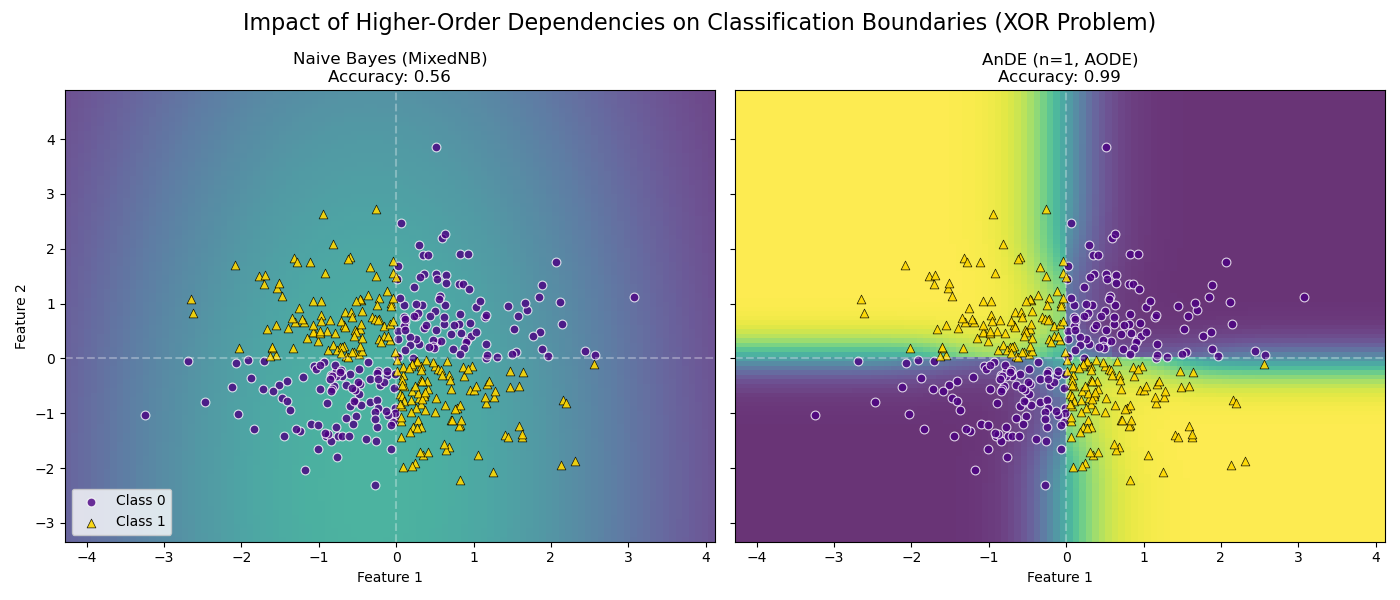
Solving the XOR Problem: AnDE vs Naive Bayes

This example demonstrates the limitations of the independence assumption in Naive Bayes and how Averaged n-Dependence Estimators (AnDE) overcome them.

We use a synthetic XOR dataset (continuous Gaussian features). In an XOR problem: - Class 0 is in quadrants 1 (+, +) and 3 (-, -). - Class 1 is in quadrants 2 (-, +) and 4 (+, -).

The Challenge: Looking at any single feature individually, the distributions of Class 0 and Class 1 overlap perfectly (both are centered at 0). Therefore, MixedNB (Naive Bayes) cannot distinguish the classes and learns a useless decision boundary (accuracy ~50%).

The Solution: AnDE (n=1) relaxes the independence assumption. By conditioning on one feature (the “super-parent”), it learns that the relationship between the other feature and the class changes depending on the parent’s value. As shown in the plot, AnDE successfully captures the XOR structure.

# Author: The scikit-bayes Developers
# SPDX-License-Identifier: BSD-3-Clause

import matplotlib.pyplot as plt
import numpy as np
from sklearn.inspection import DecisionBoundaryDisplay
from sklearn.metrics import accuracy_score

from skbn.ande import AnDE
from skbn.mixed_nb import MixedNB

# --- 1. Generate XOR Dataset (Continuous) ---
np.random.seed(42)
n_samples = 400

# Generate random points
X = np.random.randn(n_samples, 2)

# Logic: Class 0 if signs match, Class 1 if signs differ
y = np.logical_xor(X[:, 0] > 0, X[:, 1] > 0).astype(int)

# --- 2. Fit Models ---

# Model A: MixedNB (Naive Bayes, n=0)
# Expected to fail because marginal distributions are identical for both classes.
mnb = MixedNB()
mnb.fit(X, y)

# Model B: AnDE (AODE, n=1)
# Discretizes the super-parent into 4 bins (enough to capture pos/neg split)
# and models the child as a Gaussian conditioned on that bin.
ande = AnDE(n_dependence=1, n_bins=4)
ande.fit(X, y)

models = [mnb, ande]
titles = ["Naive Bayes (MixedNB)", "AnDE (n=1, AODE)"]

# --- 3. Plotting ---
fig, axes = plt.subplots(1, 2, figsize=(14, 6), sharey=True)

for ax, model, title in zip(axes, models, titles):
    # Calculate accuracy
    acc = accuracy_score(y, model.predict(X))

    # Plot Decision Boundary - VIRIDIS
    DecisionBoundaryDisplay.from_estimator(
        model,
        X,
        response_method="predict_proba",
        plot_method="pcolormesh",
        shading="auto",
        alpha=0.8,
        ax=ax,
        vmin=0,
        vmax=1,
        cmap="viridis",
    )

    # Overlay real data points with consistent style
    # Class 0 -> Indigo Circle
    ax.scatter(
        X[y == 0, 0],
        X[y == 0, 1],
        c="indigo",
        marker="o",
        s=40,
        alpha=0.8,
        edgecolors="w",
        linewidth=0.8,
        label="Class 0",
    )

    # Class 1 -> Gold Triangle
    ax.scatter(
        X[y == 1, 0],
        X[y == 1, 1],
        c="gold",
        marker="^",
        s=40,
        alpha=0.9,
        edgecolors="k",
        linewidth=0.5,
        label="Class 1",
    )

    ax.set_title(f"{title}\nAccuracy: {acc:.2f}", fontsize=12)
    ax.set_xlabel("Feature 1")

    # Add quadrant lines for reference
    ax.axvline(0, color="white", linestyle="--", alpha=0.3)
    ax.axhline(0, color="white", linestyle="--", alpha=0.3)

axes[0].set_ylabel("Feature 2")
axes[0].legend(loc="lower left")

fig.suptitle(
    "Impact of Higher-Order Dependencies on Classification Boundaries (XOR Problem)",
    fontsize=16,
)
plt.tight_layout()
plt.subplots_adjust(top=0.85)
plt.show()