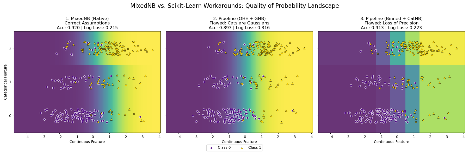
Handling Mixed Data Types with MixedNB

This example compares three strategies for handling a dataset with mixed continuous (Gaussian) and discrete (Categorical) features.

The Scenario (Generative Data):

We generate data from two natural clusters (Classes 0 and 1):

• Continuous Feature: Two overlapping Gaussian distributions. Precision is key here.

• Categorical Feature: Different category probabilities per class. Class 0 prefers Cat ‘0’, Class 1 prefers Cat ‘2’.

The Competitors:

1. MixedNB (Native): Models Gaussian as Gaussian, Categorical as Multinomial. Matches the data generation process. (Acc: ~0.920).

2. Pipeline (OHE + GNB): Treats categories as binary Gaussians. (Acc: ~0.893).

3. Pipeline (Discretizer + CatNB): Bins continuous data. (Acc: ~0.913).

Result:

MixedNB produces the smoothest probability landscape and optimal log-loss, though standard pipelines perform reasonably well on this simple problem.

# Author: The scikit-bayes Developers
# SPDX-License-Identifier: BSD-3-Clause

import warnings

import matplotlib.pyplot as plt
import numpy as np
from sklearn.compose import ColumnTransformer
from sklearn.metrics import accuracy_score, log_loss
from sklearn.model_selection import train_test_split
from sklearn.naive_bayes import CategoricalNB, GaussianNB
from sklearn.pipeline import make_pipeline
from sklearn.preprocessing import KBinsDiscretizer, OneHotEncoder

from skbn.mixed_nb import MixedNB

# Suppress warnings
warnings.filterwarnings("ignore")

# --- 1. Generate Probabilistic Mixed Data ---
np.random.seed(42)
n_samples = 1000

# Class 0: Centered at X=-1, Prefer Cat 0
n0 = n_samples // 2
X_cont_0 = np.random.normal(-1.0, 1.0, size=n0)
# Probabilities for Cat 0, 1, 2: [0.7, 0.2, 0.1]
X_cat_0 = np.random.choice([0, 1, 2], size=n0, p=[0.7, 0.2, 0.1])

# Class 1: Centered at X=1, Prefer Cat 2
n1 = n_samples - n0
X_cont_1 = np.random.normal(1.0, 1.0, size=n1)
# Probabilities for Cat 0, 1, 2: [0.1, 0.2, 0.7]
X_cat_1 = np.random.choice([0, 1, 2], size=n1, p=[0.1, 0.2, 0.7])

# Combine
X_cont = np.concatenate([X_cont_0, X_cont_1])
X_cat = np.concatenate([X_cat_0, X_cat_1])
y = np.concatenate([np.zeros(n0), np.ones(n1)]).astype(int)

# Stack: [Continuous, Categorical]
X = np.column_stack([X_cont, X_cat])

# Split for valid metric calculation
X_train, X_test, y_train, y_test = train_test_split(
    X, y, test_size=0.3, random_state=42
)

# --- 2. Define Models ---

# Model 1: MixedNB
mnb = MixedNB()
mnb.fit(X_train, y_train)

# Model 2: OHE + GaussianNB
pipe_ohe = make_pipeline(
    ColumnTransformer(
        [("onehot", OneHotEncoder(handle_unknown="ignore", sparse_output=False), [1])],
        remainder="passthrough",
    ),
    GaussianNB(),
)
pipe_ohe.fit(X_train, y_train)

# Model 3: Discretizer + CategoricalNB
pipe_kbins = make_pipeline(
    ColumnTransformer(
        [
            (
                "discretizer",
                KBinsDiscretizer(n_bins=5, encode="ordinal", strategy="quantile"),
                [0],
            )
        ],
        remainder="passthrough",
    ),
    CategoricalNB(),
)
pipe_kbins.fit(X_train, y_train)

models = [mnb, pipe_ohe, pipe_kbins]
titles = [
    "1. MixedNB (Native)\nCorrect Assumptions",
    "2. Pipeline (OHE + GNB)\nFlawed: Cats are Gaussians",
    "3. Pipeline (Binned + CatNB)\nFlawed: Loss of Precision",
]

# --- 3. Visualization ---
fig, axes = plt.subplots(1, 3, figsize=(18, 6), sharey=True)

# Grid for plotting
h = 0.05
x_min, x_max = X[:, 0].min() - 0.5, X[:, 0].max() + 0.5
y_min, y_max = -0.5, 2.5  # Categories 0, 1, 2
xx, yy = np.meshgrid(np.arange(x_min, x_max, h), np.arange(y_min, y_max, 1))

# Flatten for prediction
grid_X = np.c_[xx.ravel(), yy.ravel()]

for ax, model, title in zip(axes, models, titles):
    # Predict
    Z = model.predict_proba(grid_X)[:, 1]
    Z = Z.reshape(xx.shape)

    # Metrics on Test Set
    acc = accuracy_score(y_test, model.predict(X_test))
    ll = log_loss(y_test, model.predict_proba(X_test))

    # Plot Heatmap - VIRIDIS
    # 0.0 = Purple (Class 0 zone), 1.0 = Yellow (Class 1 zone)
    ax.imshow(
        Z,
        extent=(x_min, x_max, y_min, y_max),
        origin="lower",
        cmap="viridis",
        vmin=0,
        vmax=1,
        aspect="auto",
        alpha=0.8,
    )

    # Overlay real data points (with jitter on Y)
    X_plot = X_test.copy()
    y_jit = X_plot[:, 1] + np.random.uniform(-0.2, 0.2, size=len(X_plot))

    # Visual Coherence with Viridis:
    # Class 0 -> Indigo (Matches background purple)
    # Class 1 -> Gold (Matches background yellow)
    # Edgecolors='w' ensures visibility even on matching backgrounds

    ax.scatter(
        X_plot[y_test == 0, 0],
        y_jit[y_test == 0],
        c="indigo",
        marker="o",
        s=30,
        alpha=0.9,
        edgecolors="w",
        linewidth=0.8,
        label="Class 0",
    )

    ax.scatter(
        X_plot[y_test == 1, 0],
        y_jit[y_test == 1],
        c="gold",
        marker="^",
        s=30,
        alpha=0.9,
        edgecolors="k",
        linewidth=0.5,
        label="Class 1",
    )  # Black edge for yellow points for better contrast

    # Title & Metrics
    ax.set_title(f"{title}\nAcc: {acc:.3f} | Log Loss: {ll:.3f}", fontsize=12)
    ax.set_xlabel("Continuous Feature")
    ax.set_yticks([0, 1, 2])

axes[0].set_ylabel("Categorical Feature")
# Clean legend
handles, labels = axes[0].get_legend_handles_labels()
fig.legend(handles, labels, loc="lower center", ncol=2, bbox_to_anchor=(0.5, 0.02))

fig.suptitle(
    "MixedNB vs. Scikit-Learn Workarounds: Quality of Probability Landscape",
    fontsize=16,
)
plt.tight_layout()
plt.subplots_adjust(top=0.80, bottom=0.15)
plt.show()